新しいネットワークを書いてみよう
ここでは、MNISTデータセットではなくCIFAR10という32x32サイズの小さなカラー画像に10クラスのいずれかのラベルがついたデータセットを用いて、いろいろなモデルを自分で書いて試行錯誤する流れを体験してみます。
| airplane | automobile | bird | cat | deer | dog | frog | horse | ship | truck |
|---|---|---|---|---|---|---|---|---|---|
 |
 |
 |
 |
 |
 |
 |
 |
 |
 |
[22]:
# Install Chainer and CuPy!

!curl https://colab.chainer.org/install | sh -
Reading package lists... Done
Building dependency tree
Reading state information... Done
libcusparse8.0 is already the newest version (8.0.61-1).
libnvrtc8.0 is already the newest version (8.0.61-1).
libnvtoolsext1 is already the newest version (8.0.61-1).
0 upgraded, 0 newly installed, 0 to remove and 1 not upgraded.
Requirement already satisfied: cupy-cuda80==4.0.0b3 from https://github.com/kmaehashi/chainer-colab/releases/download/2018-02-06/cupy_cuda80-4.0.0b3-cp36-cp36m-linux_x86_64.whl in /usr/local/lib/python3.6/dist-packages
Requirement already satisfied: numpy>=1.9.0 in /usr/local/lib/python3.6/dist-packages (from cupy-cuda80==4.0.0b3)
Requirement already satisfied: six>=1.9.0 in /usr/local/lib/python3.6/dist-packages (from cupy-cuda80==4.0.0b3)
Requirement already satisfied: fastrlock>=0.3 in /usr/local/lib/python3.6/dist-packages (from cupy-cuda80==4.0.0b3)
Requirement already satisfied: chainer==4.0.0b3 in /usr/local/lib/python3.6/dist-packages
Requirement already satisfied: filelock in /usr/local/lib/python3.6/dist-packages (from chainer==4.0.0b3)
Requirement already satisfied: six>=1.9.0 in /usr/local/lib/python3.6/dist-packages (from chainer==4.0.0b3)
Requirement already satisfied: numpy>=1.9.0 in /usr/local/lib/python3.6/dist-packages (from chainer==4.0.0b3)
Requirement already satisfied: protobuf>=3.0.0 in /usr/local/lib/python3.6/dist-packages (from chainer==4.0.0b3)
Requirement already satisfied: setuptools in /usr/lib/python3/dist-packages (from protobuf>=3.0.0->chainer==4.0.0b3)
1. モデルの定義
モデルは、Chainクラスを継承して定義します。ここでは、以前試した全結合層だけからなるネットワークではなく、畳込み層を持つネットワークを定義してみます。このモデルは3つの畳み込み層を持ち、2つの全結合層がそのあとに続いています。
モデルの定義は主に2つのメソッドの定義によって行います。
- コンストラクタでモデルを構成するレイヤーを定義する
- この際、親クラス(
Chain)のコンストラクタにキーワード引数として構成するLinkオブジェクトを渡すことでOptimizerから捕捉可能な最適化対象のパラメータを持つレイヤをモデルに追加することができます。
- この際、親クラス(
()アクセサでデータを受け取り、Forward計算を行う__call__メソッドを定義する
[ ]:
import chainer
import chainer.functions as F
import chainer.links as L

class MyModel(chainer.Chain):

    def __init__(self, n_out):
        super(MyModel, self).__init__()
        with self.init_scope():
            self.conv1=L.Convolution2D(None, 32, 3, 3, 1)
            self.conv2=L.Convolution2D(32, 64, 3, 3, 1)
            self.conv3=L.Convolution2D(64, 128, 3, 3, 1)
            self.fc4=L.Linear(None, 1000)
            self.fc5=L.Linear(1000, n_out)

    def __call__(self, x):
        h = F.relu(self.conv1(x))
        h = F.relu(self.conv2(h))
        h = F.relu(self.conv3(h))
        h = F.relu(self.fc4(h))
        h = self.fc5(h)
        return h
2. 学習
ここで、あとから別のモデルも簡単に同じ設定で訓練できるよう、train関数を定義しておきます。これは、モデルのオブジェクトを渡すと、中でTrainerを用いてCIFAR10データセットの画像を10クラスに分類するようにそのモデルを訓練し、学習が終了したモデルを返す関数です。
このtrain関数を用いて、上で定義したMyModelモデルを訓練してみます。
[24]:
from chainer.datasets import cifar
from chainer import iterators
from chainer import optimizers
from chainer import training
from chainer.training import extensions

def train(model_object, batchsize=64, gpu_id=0, max_epoch=20):

    # 1. Dataset
    train, test = cifar.get_cifar10()

    # 2. Iterator
    train_iter = iterators.SerialIterator(train, batchsize)
    test_iter = iterators.SerialIterator(test, batchsize, False, False)

    # 3. Model
    model = L.Classifier(model_object)
    if gpu_id >=0:
        model.to_gpu(gpu_id)

    # 4. Optimizer
    optimizer = optimizers.Adam()
    optimizer.setup(model)

    # 5. Updater
    updater = training.StandardUpdater(train_iter, optimizer, device=gpu_id)

    # 6. Trainer
    trainer = training.Trainer(updater, (max_epoch, 'epoch'), out='{}_cifar10_result'.format(model_object.__class__.__name__))

    # 7. Evaluator

    class TestModeEvaluator(extensions.Evaluator):

        def evaluate(self):
            model = self.get_target('main')
            ret = super(TestModeEvaluator, self).evaluate()
            return ret

    trainer.extend(extensions.LogReport())
    trainer.extend(TestModeEvaluator(test_iter, model, device=gpu_id))
    trainer.extend(extensions.PrintReport(['epoch', 'main/loss', 'main/accuracy', 'validation/main/loss', 'validation/main/accuracy', 'elapsed_time']))
    trainer.extend(extensions.PlotReport(['main/loss', 'validation/main/loss'], x_key='epoch', file_name='loss.png'))
    trainer.extend(extensions.PlotReport(['main/accuracy', 'validation/main/accuracy'], x_key='epoch', file_name='accuracy.png'))
    trainer.run()
    del trainer

    return model

gpu_id = 0  # Set to -1 if you don't have a GPU

model = train(MyModel(10), gpu_id=gpu_id)
epoch       main/loss   main/accuracy  validation/main/loss  validation/main/accuracy  elapsed_time
1           1.54694     0.439258       1.30523               0.529956                  8.03004
2           1.23726     0.550636       1.17575               0.576831                  16.4374
3           1.08471     0.610075       1.14349               0.590068                  24.8839
4           0.967907    0.65505        1.10574               0.611863                  33.3805
5           0.866499    0.689218       1.07167               0.628483                  41.8358
6           0.766769    0.728293       1.09448               0.622213                  50.3215
7           0.662081    0.765485       1.06968               0.641919                  58.7635
8           0.563926    0.800456       1.14094               0.644805                  67.2734
9           0.456143    0.838895       1.2362                0.634355                  75.8304
10          0.37011     0.868478       1.36768               0.629678                  84.2881
11          0.291623    0.898508       1.4429                0.632862                  92.7059
12          0.221855    0.923075       1.61204               0.632365                  101.112
13          0.17944     0.938279       1.72657               0.632962                  109.575
14          0.151354    0.947203       1.82557               0.629279                  118.123
15          0.134023    0.953365       1.92198               0.636047                  126.677
16          0.108057    0.962848       2.1984                0.628185                  135.134
17          0.110298    0.962676       2.16424               0.629877                  143.601
18          0.106488    0.963168       2.2171                0.632763                  152.024
19          0.0853957   0.970531       2.39253               0.626393                  160.443
20          0.0873332   0.970711       2.47626               0.623905                  168.915
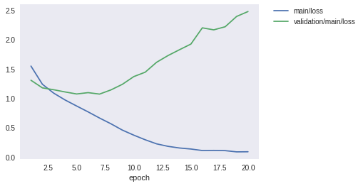
学習が一通り終わりました。ロスと精度のプロットを見てみましょう。
[25]:
from IPython.display import Image
Image(filename='MyModel_cifar10_result/loss.png')
[25]:
[26]:
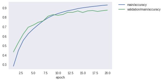
Image(filename='MyModel_cifar10_result/accuracy.png')
[26]:
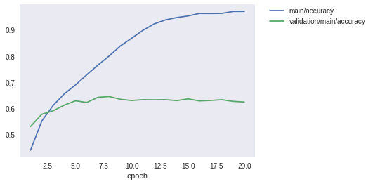
学習データでの精度は97%付近まで到達していますが、テストデータではロスはむしろIterationを進むごとに大きくなってしまっており、また精度も60%付近で頭打ちになってしまっています。モデルが学習データにオーバーフィッティングしていると思われます。
3. 学習済みモデルを使った予測
テスト精度は60%程度でしたが、この学習済みモデルを使っていくつかのテスト画像を分類させてみましょう。
[27]:
%matplotlib inline
import matplotlib.pyplot as plt
cls_names = ['airplane', 'automobile', 'bird', 'cat', 'deer',
'dog', 'frog', 'horse', 'ship', 'truck']
def predict(model, image_id):
_, test = cifar.get_cifar10()
x, t = test[image_id]
model.to_cpu()
y = model.predictor(x[None, ...]).data.argmax(axis=1)[0]
print('predicted_label:', cls_names[y])
print('answer:', cls_names[t])
plt.imshow(x.transpose(1, 2, 0))
plt.show()
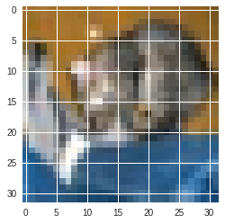
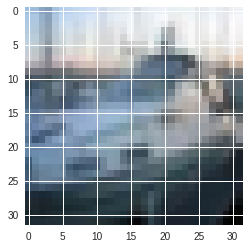
for i in range(5):
predict(model, i)
predicted_label: cat
answer: cat
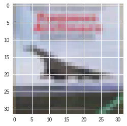
predicted_label: automobile
answer: ship
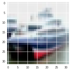
predicted_label: ship
answer: ship
predicted_label: airplane
answer: airplane
predicted_label: frog
answer: frog
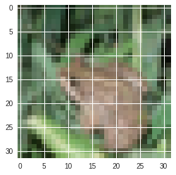
うまく分類できているものもあれば、そうでないものもありました。モデルの学習に使用したデータセット上ではほぼ百発百中で正解できるとしても、未知のデータ、すなわちテストデータセットにある画像に対して高精度な予測ができなければ、意味がありません。テストデータでの精度は、モデルの汎化性能に関係していると言われます。
どうすれば高い汎化性能を持つモデルを設計し、学習することができるでしょうか?
4. もっと深いモデルを定義してみよう
では、上のモデルよりもよりたくさんの層を持つモデルを定義してみましょう。ここでは、1層の畳み込みネットワークをConvBlock、1層の全結合ネットワークをLinearBlockとして定義し、これをたくさんシーケンシャルに積み重ねる方法で大きなネットワークを定義してみます。
構成要素を定義する
まず、今目指している大きなネットワークの構成要素となるConvBlockとLinearBlockを定義してみましょう。
[ ]:
class ConvBlock(chainer.Chain):

    def __init__(self, n_ch, pool_drop=False):
        w = chainer.initializers.HeNormal()
        super(ConvBlock, self).__init__()
        with self.init_scope():
            self.conv = L.Convolution2D(None, n_ch, 3, 1, 1,
                                 nobias=True, initialW=w)
            self.bn = L.BatchNormalization(n_ch)


        self.pool_drop = pool_drop

    def __call__(self, x):
        h = F.relu(self.bn(self.conv(x)))
        if self.pool_drop:
            h = F.max_pooling_2d(h, 2, 2)
            h = F.dropout(h, ratio=0.25)
        return h

class LinearBlock(chainer.Chain):

    def __init__(self):
        w = chainer.initializers.HeNormal()
        super(LinearBlock, self).__init__()
        with self.init_scope():
            self.fc = L.Linear(None, 1024, initialW=w)

    def __call__(self, x):
        return F.dropout(F.relu(self.fc(x)), ratio=0.5)
ConvBlockはChainを継承したモデルとして定義されています。これは一つの畳み込み層とBatch Normalization層をパラメータありで持っているので、これらをコンストラクタで登録しています。__call__メソッドでは、これらにデータを渡しつつ、活性化関数を適用して、さらにpool_dropがコンストラクタにTrueで渡されているときはMax PoolingとDropoutという関数を適用するような小さなネットワークになっています。
Chainerでは、Pythonを使って書いたforward計算のコード自体がモデルを表します。すなわち、実行時にデータがどのような層をくぐっていったか、ということがネットワークそのものを定義します。これによって、このような分岐を含むようなネットワークも簡単に書け、柔軟かつシンプルで可読性の高いネットワーク定義が可能になります。これがDefine-by-Runと呼ばれる特徴です。
大きなネットワークの定義
次に、これらの小さなネットワークを構成要素として積み重ねて、大きなネットワークを定義してみましょう。
[ ]:
class DeepCNN(chainer.ChainList):

    def __init__(self, n_output):
        super(DeepCNN, self).__init__(
            ConvBlock(64),
            ConvBlock(64, True),
            ConvBlock(128),
            ConvBlock(128, True),
            ConvBlock(256),
            ConvBlock(256, True),
            LinearBlock(),
            LinearBlock(),
            L.Linear(None, n_output)
        )

    def __call__(self, x):
        for f in self.children():
            x = f(x)
        return x
ここで利用しているのが、ChainListというクラスです。このクラスはChainを継承したクラスで、いくつものLinkやChainを順次呼び出していくようなネットワークを定義するときに便利です。ChainListを継承して定義されるモデルは、親クラスのコンストラクタを呼び出す際にキーワード引数ではなく普通の引数としてLinkもしくはChainオブジェクトを渡すことができます。そしてこれらは、self.children()メソッドによって登録した順番に取り出すことができます。
この特徴を使うと、forward計算の記述が簡単になります。self.children()が返す構成要素のリストから、for文で構成要素を順番に取り出していき、そもそもの入力であるxに取り出してきた部分ネットワークの計算を適用して、この出力でxを置き換えるということを順番に行っていけば、一連のLinkまたはChainを、コンストラクタで親クラスに登録した順番と同じ順番で適用していくことができます。そのため、シーケンシャルな部分ネットワークの適用によって表される大きなネットワークを定義するのに重宝します。
[30]:
model = train(DeepCNN(10), gpu_id=gpu_id)
epoch       main/loss   main/accuracy  validation/main/loss  validation/main/accuracy  elapsed_time
1           1.97237     0.282809       1.60959               0.432524                  53.0532
2           1.48736     0.447543       1.37107               0.531449                  106.654
3           1.23414     0.555498       1.16859               0.622412                  160.26
4           1.05247     0.6245         0.931926              0.69367                   213.86
5           0.925462    0.674532       0.938821              0.715665                  267.558
6           0.811934    0.71883        0.804659              0.744626                  368.693
7           0.705179    0.759703       0.69344               0.760052                  477.097
8           0.618222    0.792934       0.557085              0.809614                  585.21
9           0.538749    0.818434       0.530817              0.826533                  693.462
10          0.488574    0.837608       0.547517              0.819666                  801.702
11          0.440975    0.852993       0.505241              0.828324                  909.135
12          0.394701    0.867738       0.454475              0.851115                  1017
13          0.366392    0.877178       0.460453              0.850318                  1125.1
14          0.329519    0.889825       0.410546              0.865545                  1232.98
15          0.303627    0.898287       0.483188              0.848826                  1340.54
16          0.284018    0.90537        0.424268              0.865645                  1448.37
17          0.258253    0.912364       0.415589              0.869924                  1556.45
18          0.244495    0.917514       0.488768              0.859873                  1664.38
19          0.226782    0.923876       0.426225              0.867934                  1772.52
20          0.215474    0.927677       0.39808               0.873806                  1880.32
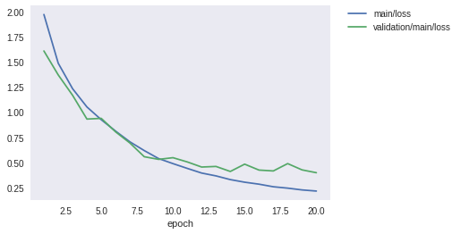
学習が終了しました。ロスと精度のグラフを見てみましょう。
[31]:
Image(filename='DeepCNN_cifar10_result/loss.png')
[31]:
[32]:
Image(filename='DeepCNN_cifar10_result/accuracy.png')
[32]:
先程よりも大幅にテストデータに対する精度が向上したことが分かります。60%前後だった精度が、87%程度まで上がりました。しかし最新の研究成果では97%近くまで達成されています。さらに精度を上げるには、今回行ったようなモデルの改良ももちろんのこと、学習データを擬似的に増やす操作(Data augmentation)や、複数のモデルの出力を一つの出力に統合する操作(Ensemble)などなど、いろいろな工夫が考えられます。